Python:Matplotlib .scatter()

The .scatter() method in Matplotlib creates scatter plots to visualize relationships between numerical variables. Scatter plots display the values of two variables as points on a Cartesian coordinate system, helping to identify correlations, patterns, and outliers in your data. This visualization tool is invaluable for data analysis, allowing researchers and data scientists to explore how changes in one variable might influence another.

Scatter plots are widely used in statistics, scientific research, and data science to examine the relationship between paired data. They’re particularly useful for detecting trends, clusters, and anomalies that might not be apparent in tabular data.

Syntax

matplotlib.pyplot.scatter(x, y, s=None, c=None, marker=None, cmap=None, norm=None, vmin=None, vmax=None, alpha=None, linewidths=None, edgecolors=None, plotnonfinite=False, data=None, **kwargs)

Parameters:

• x, y: Arrays or list-like objects representing the data point coordinates
• s: Marker size in points^2 (default: None which is interpreted as rcParams['lines.markersize'] ** 2)
• c: Marker color; can be a single color, an array of colors, or a sequence of colors (default: None)
• marker: Marker style (default: ‘o’ for circle)
• cmap: Colormap name or Colormap instance for mapping intensities of colors (default: None)
• norm: Normalize object for scaling data values to Colormap range (default: None)
• vmin, vmax: Minimum and maximum values for color scaling (useful with cmap)
• alpha: Float between 0 and 1 for the blending value/transparency (default: None)
• linewidths: Width of marker borders (default: None)
• edgecolors: Colors of marker borders (default: None which means inheriting from c)
• plotnonfinite: Boolean indicating whether to plot points with non-finite c (default: False)

Return value:

The method returns a PathCollection object.

Example 1: Creating a Basic Scatter Plot

This example demonstrates how to create a basic scatter plot with Matplotlib, visualizing the relationship between two variables:

import matplotlib.pyplot as plt
import numpy as np

# Generate random data for demonstration
np.random.seed(42)  # For reproducibility
x = np.random.rand(50) * 10  # 50 random values between 0 and 10
y = 2 * x + 1 + np.random.randn(50)  # Linear relationship with some noise

# Create a scatter plot
plt.figure(figsize=(8, 6))  # Set figure size
plt.scatter(x, y)  # Create the scatter plot

# Add labels and title
plt.xlabel('X-axis')
plt.ylabel('Y-axis')
plt.title('Basic Scatter Plot Example')

# Add a grid for better readability
plt.grid(True, linestyle='--', alpha=0.7)

# Display the plot
plt.show()

Copy to clipboard
Copy to clipboard

This code creates a scatter plot showing the relationship between randomly generated x and y values, where y has a linear relationship with x plus some random noise. The plot displays 50 data points, each represented by a circle marker.

Example 2: Customizing Scatter Plots with Size, Color, and Transparency

This example shows how to customize scatter plots by varying marker size, color, and transparency based on additional data dimensions:

import matplotlib.pyplot as plt
import numpy as np

# Generate sample data
np.random.seed(0)
x = np.random.rand(100) * 10
y = np.random.rand(100) * 10
sizes = np.random.rand(100) * 500  # Varying marker sizes
colors = np.random.rand(100)  # Values for colormapping

# Create a scatter plot with customized appearance
plt.figure(figsize=(10, 8))
scatter = plt.scatter(x, y,
                     s=sizes,  # Set marker sizes
                     c=colors,  # Set colors
                     cmap='viridis',  # Choose colormap
                     alpha=0.6,  # Set transparency
                     edgecolors='black',  # Add black edges to markers
                     linewidths=0.5)  # Set edge width

# Add labels, title, and grid
plt.xlabel('Feature 1')
plt.ylabel('Feature 2')
plt.title('Scatter Plot with Size and Color Variation')
plt.grid(True, linestyle='--', alpha=0.3)

# Add a colorbar to show the mapping of colors
plt.colorbar(scatter, label='Color Value')

plt.tight_layout()
plt.show()

Copy to clipboard
Copy to clipboard

This example creates a more advanced scatter plot where:

• The size of each marker varies based on the sizes array
• The color of each marker is determined by the colors array and the ‘viridis’ colormap
• Markers have partial transparency (alpha=0.6) and thin black edges
• A colorbar is added to explain what the colors represent

Example 3: Using Scatter Plots for Real-world Data Analysis

This example demonstrates how to use scatter plots for analyzing real-world data, specifically the relationship between height and weight in a dataset:

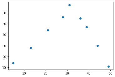
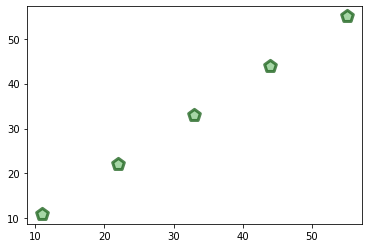
import matplotlib.pyplot as plt
import numpy as np

# Sample height (cm) and weight (kg) data for two groups
# Group 1 (e.g., males)
heights_1 = np.array([170, 175, 180, 165, 160, 185, 190, 175, 180, 185])
weights_1 = np.array([68, 72, 78, 65, 60, 85, 90, 75, 77, 85])

# Group 2 (e.g., females)
heights_2 = np.array([160, 165, 170, 155, 150, 160, 165, 155, 170, 160])
weights_2 = np.array([55, 58, 62, 53, 50, 58, 62, 51, 63, 56])

plt.figure(figsize=(10, 6))

# Create scatter plots for both groups with different colors and labels
plt.scatter(heights_1, weights_1, c='blue', label='Group 1', alpha=0.7, s=100)
plt.scatter(heights_2, weights_2, c='red', label='Group 2', alpha=0.7, s=100)

# Calculate and plot trendlines (best fit lines)
z1 = np.polyfit(heights_1, weights_1, 1)
p1 = np.poly1d(z1)
plt.plot(heights_1, p1(heights_1), "b--", alpha=0.8)

z2 = np.polyfit(heights_2, weights_2, 1)
p2 = np.poly1d(z2)
plt.plot(heights_2, p2(heights_2), "r--", alpha=0.8)

# Add labels, title, and legend
plt.xlabel('Height (cm)')
plt.ylabel('Weight (kg)')
plt.title('Height vs. Weight Comparison Between Groups')
plt.legend()

# Add grid and adjust layout
plt.grid(True, linestyle='--', alpha=0.4)
plt.tight_layout()

plt.show()

Copy to clipboard
Copy to clipboard

This example visualizes the relationship between height and weight for two different groups, possibly representing males and females. Key features include:

• Different colors to distinguish between the two groups
• Semi-transparent markers for better visibility when points overlap
• Trend lines showing the linear relationship for each group
• Appropriate labels, title, and legend to make the plot informative
• A grid to help with reading values off the chart

Frequently Asked Questions

1. How do I create a scatter plot with different colors for different categories?

To create a scatter plot with different colors for different categories, use the c parameter with a list of colors or a categorical variable, and specify a Colormap with the cmap parameter. For categorical data, you can manually assign colors to each category.

2. Can I adjust the size of the markers in a scatter plot?

Yes, you can adjust the marker size using the s parameter. This parameter accepts a single value for uniform size or an array of values for varying sizes. Note that the values represent the area of the marker in points squared.

3. How do I add a colorbar to my scatter plot?

To add a colorbar, store the scatter plot object that’s returned when you call plt.scatter(), then pass this object to plt.colorbar(). For example:

scatter = plt.scatter(x, y, c=colors, cmap='viridis')
plt.colorbar(scatter, label='Color Value')

Copy to clipboard
Copy to clipboard

4. Can I create bubble charts with Matplotlib’s scatter function?

Yes, a bubble chart is essentially a scatter plot where the marker size varies according to a third variable. Use the s parameter to set the marker sizes based on your third variable.

5. How do I control transparency in scatter plots?

Use the alpha parameter to control transparency. The value should be between 0 (completely transparent) and 1 (completely opaque). This is particularly useful when dealing with overlapping points.